
NeuroLogic: Fundamentals
EEG Fundamentals
Welcome
Read the signal, then report what it shows
This self-paced course is designed for neurology residents and clinicians beginning to read scalp EEG. Each topic combines an explanation, a model or clinical example, and a short check. Experienced readers can use individual lessons for review.
About 3 hours 35 minutes42 short lessons · learn in order or choose a topic from Contents
Before lesson 1
Take the pre-test
Answer the short pre-test before you start, and the matching post-test after the last lesson. Together they show what the course teaches you and help us improve it. A random study code pairs the two; no names or email addresses are collected.
The test link is loading.
Submit the Google Form, then come back here. Opening the link alone does not record a response.
Use a code saved on another device
By the end, you can:
- Explain where the scalp signal comes from and why a channel compares two inputs.
- Use the 10–20 map, montages, filters, and polarity to describe what appears on a page.
- Recognize common background, sleep, artifact, and abnormal patterns, then organize a report.
Course topics
From cortex to channel
Follow five steps from cortical current to recorded channel. This sequence explains polarity, montage subtraction, and the limits of scalp localization.
- Source population: Synaptic currents create graded postsynaptic potentials in cortical neurons. Single axonal action potentials are too brief and spatially scattered to dominate routine scalp EEG.
- Open field: Thousands of similarly oriented pyramidal cells must be active with enough synchrony for their extracellular fields to add instead of cancel.
- Volume conduction: The summed field spreads through brain, CSF, skull, and scalp. This passive journey attenuates and spatially blurs the signal; it does not create a new rhythm.
- Electrode potential: Each scalp electrode samples the local extracellular potential produced by the mixture of fields that reaches it. An electrode has no meaningful absolute voltage by itself.
- Channel difference: The amplifier displays Input 1 minus Input 2. The waveform therefore belongs to a channel (a comparison), not to either electrode alone.
A crowd is quiet at a distance when everyone speaks independently and loud when many people clap together. Cortical synchrony likewise emerges from interacting thalamocortical and intracortical networks; the thalamus is important for several rhythms, but it is not the sole conductor of EEG.
Scalp detection generally requires synchronous activation across several square centimeters of cortex; often-cited estimates begin around 6 cm², but detectability varies with depth, orientation, synchrony, amplitude, and competing background activity.

The diagram above traced cortex → extracellular field → volume conduction → electrode. Routine scalp EEG reflects the summed postsynaptic fields of synchronized cortical populations, not individual axonal spikes.
Quick check Follow the diagram from cortex to scalp. Which signal contributes most directly to routine scalp EEG?
Source population → open field → volume conduction → electrode potential → channel difference. That sequence is the conceptual spine of the course.
Ions, channels and membrane voltage
Every EEG signal begins as current crossing neuronal membranes. These three 20-second clips build the cellular vocabulary the rest of the course uses: why a neuron rests near −70 mV, how voltage-gated channels produce a 1‑ms action potential, and how excitatory and inhibitory postsynaptic potentials add.
Millivolts inside, microvolts at the scalp. Membrane voltages are tens of millivolts (mV): rest is about −70 mV and an action potential peaks near +30 mV. Scalp EEG is measured in microvolts (µV), roughly a thousand times smaller, because the electrode records only small extracellular currents summed across many cells and weakened by CSF, skull and scalp.
| Ion | Inside | Outside | Equilibrium potential |
|---|---|---|---|
| K⁺ | about 140 mM | 3–5 mM | about −90 to −100 mV |
| Na⁺ | 10–15 mM | about 145 mM | about +60 to +70 mV |
| Cl⁻ | 4–10 mM | about 110 mM | about −65 to −90 mV |
| Ca²⁺ | about 0.0001 mM | about 2 mM | above +120 mV |
Where these ideas return
- Potassium sets rest. Because resting permeability is dominated by K⁺, a rise in extracellular K⁺ during intense firing depolarizes neighboring neurons and favors seizure spread.
- Sodium-channel inactivation sets refractoriness. Carbamazepine, phenytoin and lamotrigine stabilize the fast-inactivated state; lacosamide enhances slow inactivation.
- GABA-A receptors are Cl⁻ channels. Benzodiazepines and barbiturates act here. In immature neurons, high intracellular Cl⁻ can make GABA depolarizing, one proposed but debated reason these drugs work less reliably in neonatal seizures.
- Postsynaptic potentials outlast action potentials. Their long, overlapping currents are what summate into the scalp EEG, the subject of the next two lessons.
Replay the first clip: the voltage falls toward EK when K⁺ leak channels open, and only a small Na⁺ leak pulls it back toward −70 mV.
Quick check A cortical neuron rests near −70 mV. Which process sets most of that voltage?
Rest sits near EK because K⁺ leak dominates resting permeability. That is why extracellular K⁺ accumulation depolarizes neurons, and why the action potential ends as K⁺ channels open.
Continue the board-level review in How seizures start and stop.
Why EEG sees synapses, not single-neuron spikes
Routine scalp EEG is dominated by the extracellular fields of synchronized cortical postsynaptic currents. Duration helps explain temporal summation, but spatial alignment, cancellation, source extent, depth, and the competing background also determine detectability.
Predict: keep the cells aligned and increase their timing spread. Which event loses more of its summed peak: a brief biphasic action-potential-like event or a longer postsynaptic event?
The model below runs both events side by side. Each panel shows twelve model cells, standing for a much larger population, and the sum a distant electrode would receive.

Drag the timing spread from 0 to 5 ms and watch the right panel, then flip half the cells. Timing dispersion and geometric cancellation are different mechanisms. Watch what each does to the two sums.
Snapshot: at the combined peak
Sum keeps of its aligned height
Sum keeps of its aligned height
Each row is one model cell; a filled dot means it is active at the cursor. The bottom trace is the sum of the rows above it, in relative field units, not membrane voltage. Replay sweeps 120 ms in six seconds.
Why routine scalp EEG is dominated by postsynaptic fields
Brief axonal events have unfavorable temporal and spatial summation at the scalp. A quiet trace does not imply silent neurons. Likewise, synchrony is not itself epileptiform: alpha rhythms and sleep graphoelements also reflect organized population activity.
Two meanings of “spike.” A single axonal action potential lasts about 1 ms. An EEG spike is a 20–70 ms scalp waveform generated by a population of neurons. The terms describe different levels of physiology.
From ion flow to EEG polarity
Start with the extracellular space, because that is where the EEG electrode listens. A sink is a membrane region where conventional positive current enters the neuron. Removing positive charge makes the nearby extracellular space relatively negative. A source is the return-current region, where positive current leaves the cell and the extracellular space becomes relatively positive.
Pyramidal cells are aligned perpendicular to the cortical surface. When many of them activate together, the sink and source fields add as an open field. Move the synaptic current from the apical dendrites to the soma and the dipole flips, even though the cellular event can still be excitatory.
Try: switch EPSP and IPSP, then move the synapse from apical dendrite to soma. Watch the extracellular sign and the scalp deflection change together.
Move the synapse, then follow the charge
EEG deflection
Compared with a fixed, quiet reference.
Schematic shape, not a measured voltage.
About this model
This figure represents an aligned population of pyramidal cells, with a fixed quiet reference. The return current is distributed across the membrane; its arrows show a simplified circuit.
The EPSP example uses inward Na+ current. The IPSP example uses inward Cl− current at a mature, hyperpolarizing synapse. Inhibition depends on ionic driving force and conductance, so polarity alone does not identify excitation, inhibition, or a neurotransmitter.
Keep the order straight: identify where current crosses the membrane, decide whether the nearby extracellular space is a sink or source, determine the dipole orientation, and only then predict the scalp polarity. Clinical EEG displays relative negativity upward.
Use the polarity rules and ion lab above: inward positive current at a superficial synapse removes positive charge from the nearby extracellular space, leaving relative negativity at the electrode.
Quick check Positive current enters a superficial apical dendrite during an EPSP. What does the nearby extracellular electrode sample?
Current in removes positive charge from the extracellular space. The sink is therefore relatively negative. Return current creates a source elsewhere, and the separation forms the dipole.
Continue the board-level review in What the scalp can see.
Dipole orientation and scalp maxima
Pyramidal cells stand perpendicular to the cortical surface, and the cortex is folded, so the fold decides which way the dipole points. A cell on a gyral crown points its dipole up at the scalp. A cell on a sulcal wall points sideways. Orientation changes the scalp field. The field maximum alone cannot uniquely determine the generator.
Try these three comparisons:
- Change orientation: select Radial, Oblique, then Tangential. Watch where the largest field moves and compare the Electrode overhead reading.
- Change depth: return to Radial and increase Source depth from 1.0 to 2.0. Watch the curve and the Peak strength reading.
- Compare two sources: reset depth to 1.0, then toggle Add an opposing source. Compare the field’s strength and shape with one source versus two.
How the cortex sets orientation
Radial · toward the scalp
Where the scalp field is largest
Blue −, upward · Red +, downward
About this model
The fold illustrates orientation; the depth slider separately controls source depth in relative units. The added source has equal strength, opposite orientation, and a fixed separation of 0.4 units. It is shown in the field panel.
Point dipoles in a homogeneous conductor, with zero reference at infinity. Field units are relative, not microvolts; the radial peak at depth 1 is 100 units. Electrode colors show polarity. Source symbols are schematic. A scalp maximum cannot uniquely locate a cortical source.
At 90° in this model: the field is zero directly above the source, with opposite-polarity peaks on either side. Neither peak alone locates the underlying cortical generator.
Why deep sources hide
Greater depth reduces and broadens the field in this model. Opposing cortical populations can partially or completely cancel, depending on their relative timing, strength, and geometry. Orientation and depth are separate variables; neither alone determines scalp detectability.
EEG and MEG provide complementary views. In a spherical approximation, MEG is preferentially sensitive to tangential sources, while EEG detects radial and tangential components. Real anatomy and noise also affect both recordings.
Once the field reaches the scalp, the next task is naming the electrode sites that sample it.
The international 10–20 map
The International 10-20 system turns four reproducible landmarks into a proportional scalp map. Electrode sites fall at 10% and 20% intervals, so the same labels can be applied across different head sizes. A label is a scalp coordinate, not a promise that the same cortical gyrus lies directly beneath it in every patient.
Vertex view of the scalp map

The four landmarks that anchor the map
Reference, ground, and contact: A1/A2 are auricular sites; M1/M2 are mastoids. Check electrode-skin impedance before recording and when artifact appears. ACNS guidance ordinarily keeps it at or below 5 kΩ, balanced across the array, but a near-zero reading can indicate a salt bridge that shorts adjacent electrodes together.
Test the map now. Lead Placement is the next lesson, while these locations are still fresh.
Review the full technical framework in Recording technique.
Bipolar montages and phase reversal
Voltage is measured between two points. An EEG channel displays the difference between its two inputs: Input 1 − Input 2.
An EEG montage is a logical display of differential channels. The longitudinal bipolar ("double banana") montage is an essential standard display, but no single montage is sufficient for every pattern. Clinical review uses complementary bipolar and referential displays and preserves the ability to reformat digitally.
Clinical page (first half)

- Left temporal
- Right temporal
- Left parasagittal
- Right parasagittal
- Midline
Montage layout

Common Mode Rejection (CMR): Differential amplifiers reject signals that affect both inputs equally (like line-frequency ambient hum) and amplify only the difference between Input 1 and Input 2. This is what lets a microvolt-scale cerebral rhythm survive alongside environmental interference that can be several orders of magnitude larger at the electrode.
Phase reversal is created by a shared electrode
In a bipolar montage, neighboring electrodes form a chain. For example, Fp1–F3 and F3–C3 share F3, but F3 is Input 2 in the first channel and Input 1 in the second.
Channel output = Input 1 voltage − Input 2 voltage
If Input 1 is −50 μV and Input 2 is −20 μV:
(−50 μV) − (−20 μV) = −30 μV (an upward deflection, because negative is up).
Follow the shared electrode
When a focal negative field is maximal at F3, it becomes the most negative point in the surrounding chain:
- Channel 1 (Fp1–F3): F3 is Input 2. Since Input 2 is the more negative input, the subtraction formula outputs a positive value (Fp1 − F3 = (−20) − (−100) = +80 μV). The channel deflects downward.
- Channel 2 (F3–C3): F3 is Input 1. Since Input 1 is the more negative input, the formula outputs a negative value (F3 − C3 = (−100) − (−25) = −75 μV). The channel deflects upward.
This creates a converging phase reversal at the negative chain maximum. A positive field creates a diverging reversal. A reversal localizes a voltage maximum in that chain; it does not, by itself, prove epilepsy or guarantee that the cortical generator lies directly beneath the electrode.
The shared electrode is the one that reverses
Left parasagittal chain, with a surface-negative discharge maximal at F3
Bipolar math: five electrodes, four channels
Now isolate the arithmetic from the terminology. Change one electrode at a time and keep the five electrode voltages, all four subtractions, and all four traces visible together. Then apply the same reasoning to the clinical page immediately below.
1 / 9
Five electrodes, four channels. Each interior electrode is shared by the two channels either side of it; that is what makes a reversal possible.
Ch1 Fp1–F3
Ch2 F3–C3
Ch3 C3–P3
Ch4 P3–O1
Bipolar practice: find the reversal
Two skills from the bipolar math lab, now on real pages. First, walk each chain until two neighboring channels deflect toward each other; the electrode they share is a local negative extremum along that chain. Second, read the channel list itself: front-to-back pairs in temporal, parasagittal, then midline chains name the double banana.
A phase reversal is not the biggest deflection on the page. It is two adjacent channels in the same chain turning to face each other because their shared electrode is more negative than its neighbors.
Spot check A real longitudinal bipolar page: the same double banana, on an actual recording. One sharp wave repeats through it. Tap or click the chain where two channels turn to face each other.

The reversal is at F8. Walk the right temporal chain down: Fp2–F8, F8–T8, T8–P8, P8–O2. The two channels that share F8 deflect against each other, identifying F8 as more negative than its immediate neighbors in this chain, so it drives Fp2–F8 one way and F8–T8 the other. T8–P8 and P8–O2 follow F8–T8 in the same direction, only smaller: the field falls away behind F8 without turning again.
A bipolar reversal follows from a shared electrode entering adjacent channels with opposite signs. In a referential montage, Input 2 is shared throughout. Opposite referential deflections can still represent opposite field polarities.
Longitudinal chains run front to back; transverse rows run left to right; circumferential closes a ring; referential labels pair single electrodes with one reference.
Spot check Ignore the blink and read the channel list on the left. What montage is this page?

Longitudinal bipolar, the double banana. Left temporal over right temporal, then left parasagittal over right parasagittal, then a short midline chain. Each channel is a neighboring pair subtracted front to back.
Name the montage from its channel labels and connections. A blink or other waveform does not change the montage.
Referential montages and common average
Bipolar channels can attenuate a broad field when neighboring electrodes have similar voltages. A referential view provides another way to inspect the same distribution.
In a referential montage, each active scalp electrode is compared with a shared reference. A common average reference (CAR) is one useful computed option, not a universally superior standard:
- Mathematical average: CAR sums the potentials of all active scalp electrodes (19 in the standard 10-20 array) and divides by the total number, creating a computed baseline reference.
- Amplitude and field distribution: The largest deflection helps identify the scalp maximum of a field, but source orientation, depth, reference composition, and volume conduction prevent a simple one-to-one equation between amplitude and generator proximity.
- Reference contamination: If a single electrode suffers a massive artifact (e.g., a loose electrode or localized muscle spike), that high voltage is mathematically distributed into the common average, causing a "paradoxical" ghost artifact to appear across every other channel.

Full EEG page · common average reference
Montage practice: change the reference

The schematic shows the same voltages wired two ways. In bipolar, an interior electrode enters adjacent channels with opposite signs. In referential, the reference occupies Input 2 throughout. Opposite polarities may still mark opposite lobes of a field.
The bipolar shared-electrode reversal mechanism needs adjacent channels sharing one electrode at opposite amplifier inputs. Referential channels share the average at Input 2. The bipolar reversal mechanism disappears, but the field can still contain positive and negative regions.
Spot check Compare the two views of the same field. What changes when the event is re-read against one reference?
Distinguish bipolar reversal logic from opposite polarities across a field. Each referential channel is electrode − reference. The reference is shared at Input 2. A two-lobed field or an active reference can produce opposite-signed deflections; the bipolar shared-electrode rule does not apply to those rows.
In bipolar, compare adjacent channel deflections. In referential, compare signed amplitudes across neighboring electrodes. Both views help describe the scalp field relative to the chosen inputs.
Use both views: bipolar subtraction can hide a broad field, while activity in a shared reference changes every referential channel.
After choosing which voltages to compare, display settings determine how those differences appear on the screen.
Transverse and circumferential montages
Longitudinal chains run front to back, so they leave two gaps: a focus at a chain end has only one neighbor, and, without a midline chain, a midline focus is split across left and right chains. Transverse rows run left to right, so a midline field can sit inside a single chain. Circumferential closes the rim into a ring, giving occipital and frontopolar sites neighbors on both sides. Both layouts still use the same 10–20 array.
Read the EEG labels, then follow the map
Full EEG page · select to enlarge
- Frontopolar
- Frontal
- Central
- Parietal
- Occipital
- Left
- Posterior
- Right
- Anterior
Montage layout
One discharge, four montages
A montage chooses which electrode voltages to subtract. The same discharge can appear differently across montages, so compare more than one arrangement.
In this model, each montage is calculated from the same scalp field. Switching views changes the channel comparisons; the source stays in place.
left temporal over right temporal, then left parasagittal over right parasagittal; no midline chain
Field variants, reference options, and voltage table
Fixed linear voltage scale with a 50 µV calibration marker. The scalp field is illustrative and does not change when you switch montage. An active reference changes referential channels; it cancels from bipolar differences.
The same right temporal sharp wave on four real pages. Switch montage; the generator does not move.
Clinical page, windowed on the discharge (tap for the full page)
- Frontopolar
- Frontal
- Central
- Parietal
- Occipital
- Left
- Posterior
- Right
- Anterior
Montage layout
Electrode minus average. Every channel shares Input 2. Opposite polarities may occur, but they do not follow the bipolar shared-electrode reversal rule.
Read amplitudes. Compare signed amplitudes and neighboring gradients to identify the scalp field maximum relative to this reference. Here, F8–Avg and T8–Avg stand above their neighbors.
Watch the reference. One bad electrode contaminates the average and can ghost across every other channel.
Try the occipital example. O1 is at the end of the longitudinal chain. In the circumferential ring it has neighbors on both sides, allowing its field to produce a complete shared-electrode reversal.
Filters and sensitivity
Start with a normal EEG background plus slow drift, fast noise, and 60 Hz interference. Change one control at a time to reveal each artifact; sensitivity changes only its displayed height.
Normal background with artifacts in the source. Lower LFF to 0.1 Hz for slow drift, raise HFF to 150 Hz for fast noise, or turn the notch off for 60 Hz interference.
Synthetic normal background, 10 seconds. Slow drift: 0.18–0.32 Hz; fast noise: 125–190 Hz; line interference: 60 Hz. Both views use the same sensitivity and time scale. On small screens, scroll across the trace.
How to read the controls
LFF is a high-pass filter: 1 Hz reduces the slow drift in this example. HFF is a low-pass filter: 70 Hz reduces the fast noise. Neither cutoff is a brick wall, so some artifact can remain. These artifacts occupy separate bands to make the controls easy to learn; real muscle artifact also overlaps brain frequencies. Filters can attenuate useful brain activity too.
Notch: reduces activity near 60 Hz, including any brain signal in that band. Troubleshoot electrode contact and interference before relying on it. Read about digital EEG filters.
Sensitivity: divide voltage by µV/mm to find height on the teaching grid. A 70 µV wave occupies 10 mm at 7 µV/mm and 5 mm at 14 µV/mm. These are calibrated display units, not physical screen millimeters.
What each setting keeps
Troubleshoot before filtering
Use channel distribution to identify the shared bad electrode, correct the contact or environmental source, and only then adjust the display. These two checks apply that sequence.
Shared-electrode rule: list the noisy channels, find the electrode they have in common, then confirm that electrode appears in no clean channel. This distribution favors a shared electrode or its input; hardware faults need not affect every channel.
Spot check Two channels on this page are buried under a 60 Hz buzz and the rest are clean. The affected pair is Fp1–F7 and F7–T7. Which electrode is the problem?
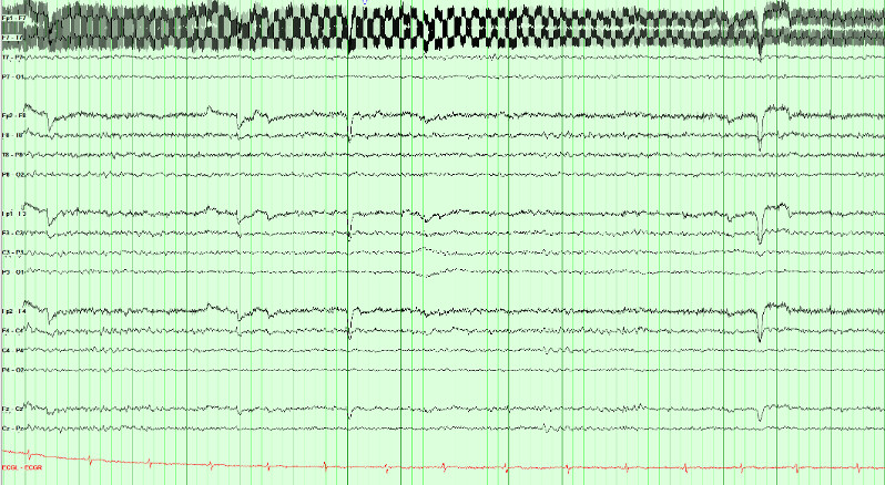
Find the electrode the noisy channels share, and check it appears nowhere clean. Fp1–F7 and F7–T7 both contain F7; Fp1 also sits in a clean Fp1–F3 and T7 also sits in a clean T7–P7. Only F7 is implicated by every channel it touches. A loose or drying F7 contact with high impedance is a likely explanation. Confirm with contact and impedance checks; the waveform alone does not prove the cause.
Check F7 contact and its lead, reduce nearby interference, and reassess. A notch may reduce residual 60 Hz activity, but it does not repair the contact and also attenuates signal near that frequency.
This is the general rule for localizing any single-electrode problem, including hum, an electrode pop, or a flat channel: list the channels that show it and take the electrode they have in common.
Sweat artifact lives below about 0.5 Hz and is often largest frontally. The low-frequency filter can attenuate it on the display, but re-gelling and cooling fix the source. A notch filter targets mains frequency, not baseline sway.
Spot check A different technical problem: the baselines on this page are swaying slowly, well below 1 Hz, and the sway is largest frontally. Which setting can attenuate it on the display while you correct the cause?
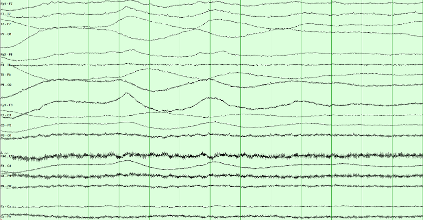
Sweat artifact occupies the lowest frequencies, so the low-frequency filter can attenuate it on the display. Sweat and slow changes in skin potential often produce sway below about 0.5 Hz. Raising the low-frequency filter modestly may improve readability, but it can also attenuate genuine cerebral delta.
Address the source: cool the patient and dry the scalp as appropriate. Then reassess the trace. Excessive low-frequency filtering can hide cerebral slowing along with sweat artifact.
Muscle artifact contains broad-band activity, including fast components. Lowering the high-frequency filter may reduce it but can also blunt cerebral sharp waves.
Digital recording: what is retained
The analog signal and sampling rate determine what a digital EEG retains. Display settings cannot restore removed frequencies, clipped voltages, or information lost through aliasing.
Acquisition chain
What acquisition preserves
The signal passes through a differential amplifier and an analog anti-alias filter before analog-to-digital conversion (ADC). Display processing then operates on those stored samples.
Still analog
-
1
Differential amplifier Input 1 minus Input 2. Common-mode interference is rejected here, not later on the screen.
-
2
Analog anti-alias filter A low-pass that must act before sampling. It attenuates frequencies that could alias at the selected sampling rate.
Already a file
-
3
Digital filtering and display LFF, HFF, notch, sensitivity, and montage reformatting. Review filters change the view of retained original samples. Processing that overwrites or discards data cannot be undone.
Information that cannot be recovered
- Content the analog anti-alias filter already removed
- The true frequency of an aliased oscillation
- Headroom, if the converter saturates
Settings you can change during review
- Display LFF, HFF, and notch
- Sensitivity, paper speed, and montage
- Review filters when the original samples were retained
Can the samples preserve the signal?
The gray curve is a 60 Hz signal; blue dots are the stored samples. Sampling does not have to land on each peak. It needs a rate above twice the highest retained frequency, with anti-alias filtering before sampling. Select 120 Hz: the dots start at the zero crossings, so the recorded values are all zero. Then move the phase slider to see why exactly two samples per cycle is unreliable.
True 60 Hz Stored samples, joined for display Wave the samples imply
Impedance is a pattern, not one number
Routine electrode–skin impedances are ordinarily kept at or below about 5 kΩ and reasonably balanced. A near-zero value suggests a salt bridge. A high or mismatched contact weakens common-mode rejection. Trace a disturbance through every channel sharing the electrode before blaming the amplifier.
Electrical safety
Use approved isolated EEG equipment, hospital-grade grounded outlets, intact short leads, and one common patient ground according to local policy. Never create extra paths to ground through other appliances. Stop to investigate damaged cables, unexpected shocks, or equipment faults.
Check acquisition first. Inspect the patient, electrodes, environment, and analog signal before adjusting display filters.
With the acquisition chain understood, the next step is learning the frequency and amplitude language used to describe the recorded waveforms.
Frequency: the four primary bands
Interpretation foundation
EEG: A Language of Its Own
Every tracing begins with frequency, the number of cycles per second in hertz, and amplitude, the voltage difference in microvolts. Those measurements become meaningful only after you add location, morphology, state, symmetry, and reactivity.
Describe frequency in hertz, then add amplitude, location, and state. These examples use the same sensitivity and illustrate decreasing amplitude as frequency increases.
Band edges follow the usual convention: 8 Hz is alpha, not theta, and 13 Hz is still alpha, not beta; beta begins above 13 Hz. Amplitude decreases automatically as you increase frequency. You can adjust voltage separately; changing frequency restores the example amplitude.
Frequency does not require a particular voltage. To compare bands at equal amplitude, select a frequency and then adjust its voltage. A posterior dominant rhythm also requires the appropriate location, state, and reactivity.
Background reactivity: The posterior dominant rhythm normally attenuates with eye opening. Reactivity is interpreted alongside state, medications, technique, and the rest of the recording; absent or reduced reactivity can be concerning but is not diagnostic in isolation.
Amplitude and voltage scales
Amplitude is measured in microvolts (µV). Sensitivity, in µV/mm, determines display height: a lower setting makes the same signal taller; a higher setting makes it shorter. The lab measures peak-to-peak amplitude.
Calibrated display lab
Separate voltage from display height
Change the selected voltage, then change sensitivity. Compare all three signals at the same display scale.
Each small grid square represents 5 mm on this teaching display. Brackets measure peak-to-peak height; these are not physical screen millimeters.
Amplitude changes when the underlying voltage changes.
Sensitivity changes only how tall every signal looks on screen.
Review display standards in Recording technique.
Intracranial vs. Scalp Voltages: Potentials recorded directly from the cortical surface are substantially larger than those at the scalp, often by roughly one to two orders of magnitude. Volume conduction through CSF, skull, and scalp both attenuates and spatially blurs the signal, which is why an intracranial electrode can resolve a discharge that the scalp never registers.
Phases, morphology, and rhythmicity
Describe a waveform with both measurements and words: frequency, amplitude, phases, shape, and repetition. Interpret those features together with its field and the patient’s state.
Phases: count the crossings
A phase is one excursion to one side of the baseline. You count phases by counting baseline crossings, not peaks; a wave with three phases crosses twice. Spikes and sharp waves are usually diphasic or triphasic; a discharge with many phases is polyphasic.
Three phases and “triphasic morphology” are not interchangeable. ACNS uses triphasic morphology as a specific modifier, commonly in GPDs. Count phases first, then assess the full waveform pattern and distribution.
One wave, or a run of them?
Polymorphic activity varies in shape from wave to wave. Monomorphic activity has a relatively uniform shape. Next, assess whether the waves repeat with a regular interval.
For ACNS rhythmic or periodic terminology, a pattern must continue for at least six cycles. The key distinction is the interval between waves:
- Periodic: discrete discharges with a measurable interval between the end of one and the start of the next.
- Rhythmic: each wave runs straight into the next, with no interval at all.
Current ACNS terminology does not use the older quasi-periodic or quasi-rhythmic modifiers. A pattern remains periodic or rhythmic when cycle length varies by less than 50% across most consecutive cycle pairs; greater variation falls outside those labels.
Build the name in two steps: describe the distribution (for example, lateralized or generalized), then the pattern (periodic discharges or rhythmic delta activity). Add the relevant modifiers afterward.
Background organization: three comparisons
Start with the background before looking for isolated events. A record can be abnormal without any epileptiform discharges. Establish the patient’s state, then work through these four questions:
- Organization: Continuous, symmetric, and does it have an anterior–posterior gradient?
- Posterior dominant rhythm: Present, in range, and symmetric; does it react?
- Variability and reactivity: Does the tracing change on its own, and change when you stimulate?
- State: Awake, drowsy, or asleep? Everything else is judged against the answer.
Use the three comparisons below to judge organization before measuring the posterior rhythm or interpreting individual transients.
Continuity
Look for sustained lower-voltage intervals interrupting the background. Interpret them with age, state, medications, and recording quality. Premature neonatal discontinuity has a different maturational meaning.
At the same montage and scale, identify lower-voltage intervals. Measure their duration and proportion before assigning a continuity category.
Symmetry
The two hemispheres should broadly match in amplitude and frequency. Compare homologous chains, not a single channel against memory.
A persistent left–right difference deserves closer review. Compare frequency and voltage across homologous regions, and check technique, state, and skull-related effects.
Anterior–posterior gradient
In a relaxed, awake adult, anterior activity is usually faster and lower in amplitude than the posterior rhythm. Assess this gradient with the eyes-closed background.
An indistinct gradient can reflect reduced organization, but also changes in arousal, medication effects, or technique. Interpret it with the rest of the background.
The posterior dominant rhythm
The PDR is a reactive occipital rhythm in an awake person with the eyes closed. Alpha names a frequency band. PDR names a finding with a location, behavioral state, and response to eye opening. Follow the complete longitudinal bipolar page before measuring it.
10-second longitudinal bipolar page
Watch the PDR appear, settle, and attenuate
The posterior temporal and parasagittal derivations are highlighted only when the finding is established.
Count the stable left posterior rhythm, compare the right, then check eye-opening reactivity. Select a count and choose Check answer.
Count the cycles
At Stable PDR, how many cycles fit between the green lines?
The bracket spans one second, so the cycle count equals the frequency in Hz.
Clinical page (first half)

Where to measure
Occipital maximum. After the mixed-frequency stretch on the left, a regular posterior alpha rhythm appears and stays maximal at O1/O2.
Measure a stable segment. Use the green one-second bracket in the model above. On the separate clinical page, use its own time markings to estimate frequency.
Still normal. Assess frequency together with posterior distribution, symmetry, state, and eye-opening reactivity.
Continue with PDR maturation in From preterm to adolescence and normal lookalikes in Normal variants that look epileptiform.
Measurement traps and adult asymmetry thresholds
Alpha squeak: the first second after eye closure may briefly run faster. Measure the stable awake segment that follows.
Drowsiness: the rhythm may look clearer but slow as arousal falls. Use the best awake sample.
Reactivity: attenuation with eye opening helps establish that the posterior rhythm is a PDR.
| Measure | Expected adult finding | Concerning difference |
|---|---|---|
| Frequency | 8–13 Hz in an awake adult | Below 8 Hz while fully awake |
| R vs L frequency | Within 1 Hz | Persistent difference greater than 1 Hz |
| R vs L amplitude | Right may be up to about 50% higher | Persistent left excess or right excess beyond about 50% |
Variability, reactivity, and state
Sedation, temperature, and impaired arousal can reduce variability and reactivity. In critical illness, interpret these findings with the full clinical assessment and other prognostic tests.
Provoke it
Interpret by wake–sleep state
Identify wakefulness, drowsiness, or sleep before interpreting slowing. Persistent delta in a fully awake adult has a different meaning from delta during N3 sleep.
Age-related findings not to over-read
| Finding | What it is |
|---|---|
| Posterior slow waves of youth | 2.5–4.5 Hz mixed into the posterior rhythm in children and adolescents, attenuating with eye opening |
| Slow / fast alpha variant | Half or double the alpha frequency; both react like alpha, and that reactivity is what identifies them |
| Benign temporal slowing | Scattered temporal theta or delta in the elderly |
Practice: assess the adult background
Apply the four background questions from the pages above: organization, PDR, reactivity, then state. The technologist has already told you this patient is awake with eyes closed and not drowsy. Read the posterior chains for the rhythm, not the frontal muscle.
Judge continuity, symmetry, and slowing on the posterior background. Frontal muscle is fast and can make a slow record look normal if you read the wrong place.
Spot check This is a fully awake adult during sustained eyes-closed recording; drowsiness has been excluded. You have run the four background questions on the page. How would you describe it? (There is muscle on the frontal channels; read past it.)
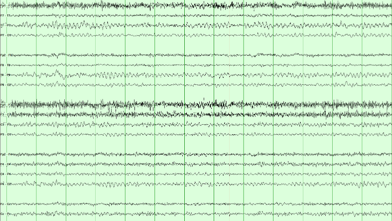
Diffuse, symmetric, continuous slowing. The background is theta-dominant across the page rather than alpha-dominant posteriorly, both hemispheres look alike, and there are no periodic or rhythmic runs. That combination is mild diffuse slowing, the commonest abnormal EEG finding there is.
It is non-specific on its own. Diffuse slowing says cerebral function is abnormal in this known-awake adult; it does not say why. Toxic, metabolic, postictal, infectious, and degenerative processes may look like this. If behavioral state were unknown, drowsiness could mimic the appearance and would have to be excluded before calling it abnormal.
Frontal muscle activity can obscure the slower cerebral background in this example. Use the less contaminated posterior regions to assess its dominant frequency.
The PDR is an occipital rhythm in an awake person with eyes closed. After a mixed opening, measure frequency and symmetry at O1 and O2, not through frontal artifact.
Spot check Awake adult, eyes closed after a mixed-frequency stretch. Where is the posterior dominant rhythm maximal?
The PDR is an occipital rhythm. After the first seconds of mixed activity, a regular alpha-range oscillation appears and stays maximal at O1 and O2. Measure it there, on the stable eyes-closed stretch, not through the frontal muscle.
Frequency, symmetry, and reactivity are the three questions that follow. Count cycles in a one-second bracket on the posterior channels; compare left with right; then confirm that eye opening attenuates it.
How normal EEG changes with age
The adult rules in this course are not universal across development. Interpret pediatric and neonatal EEG against postmenstrual age in neonates, chronological age in older children, behavioral state, and sleep–wake organization before calling slowing or discontinuity abnormal.
Pediatric PDR maturation
| Approximate age | Expected milestone |
|---|---|
| ~4 months | Posterior rhythm around 4 Hz |
| ~1 year | Posterior rhythm around 6 Hz |
| ~3 years | Posterior rhythm around 8 Hz |
| ~8 years onward | Adult-range 8–13 Hz PDR |
Sleep spindles appear at roughly 6–8 weeks and may remain asynchronous until about 2 years. Posterior slow waves of youth can be normal when they remain tied to the reactive posterior rhythm.
Neonatal preview
In neonates, state and continuity are maturational variables. Tracé discontinu is expected at very premature ages; delta brushes peak before term; tracé alternant belongs to term quiet sleep; and wakefulness/active sleep should become continuous by term. A pattern normal at 29 weeks postmenstrual age may signal severe dysfunction in an adult.
This is orientation, not neonatal interpretation training. Continue to From preterm to adolescence and Neonatal seizures in Board Review for age-specific patterns, neonatal seizures and recording standards.
Recognizing sleep architecture
Recognize sleep architecture before classifying sharp transients. NREM sleep can activate epileptiform discharges, and normal sleep waveforms can look sharp. The drawn pages share one time base and sensitivity, with the channels carrying the finding highlighted; the montage buttons re-derive the same field. N2 and N3 are recordings.
N1: light sleep
In people with a waking alpha rhythm, N1 begins as lower-amplitude mixed-frequency activity replaces it for more than half the epoch. Look for these supporting features:
- Vertex waves: brief, surface-negative sharp transients with a midline central maximum, usually near Cz.
- Slow rolling eye movements: gentle, slow horizontal oscillations.
Read the field: a vertex wave can produce reversals near C3 and C4 in longitudinal bipolar channels. Those reversals reflect the sampled field and do not establish two separate generators.
Compare montages: select Transverse to include Cz in the central chain. A reversal there better demonstrates the midline maximum. Localization depends on electrode coverage as well as subtraction.
N2: spindles and K-complexes
Recognize two characteristic N2 waveforms:
- Sleep spindles: 11–16 Hz runs, usually 12–14 Hz, lasting at least 0.5 seconds and typically largest centrally.
- K-complexes: a distinct negative sharp component followed by a positive component, with total duration at least 0.5 seconds and a frontal maximum. They may follow a stimulus.
Recognition clues: A K-complex is a sharp negative followed by a slow positive, and a spindle is a brief 11–16 Hz waxing-and-waning run. Their state-appropriate morphology, distribution, and relationship to the surrounding sleep architecture identify them; lack of evolution alone does not exclude every electrographic seizure.
N3: slow-wave sleep
Deep NREM sleep. In adults, N3 is scored when slow-wave activity at 0.5–2 Hz and at least 75 μV measured over the frontal derivations occupies at least 20% of a 30-second epoch. Other activity may still be present; spindles can occur and are not scored separately from the N3 epoch.
Recognition clues: The delta is generalized but frontally maximal; a completely uniform field would cancel out in a bipolar chain and show nothing at all.
REM: rapid eye movement sleep
REM sleep has a low-voltage, mixed-frequency background, rapid eye movements, and reduced tonic chin EMG. Brief muscle activity may still occur.
- Sawtooth waves: triangular 2–6 Hz waveforms, often central, that can precede rapid eye movements.
- Rapid eye movements: irregular conjugate movements producing prominent deflections in eye-sensitive channels.
Formal REM staging uses EEG, eye movements, and chin EMG together.
Recognition clues: The eye movements are rapid here, not the slow rolling drift of N1: each saccade is a near-vertical edge, and the left and right frontal chains are mirror images at the same instant. The sawtooth waves in Fz–Cz and Cz–Pz arrive just before each burst. There are no spindles, K-complexes or vertex waves.
Sleep practice: stage and field
Use the sleep features as a checklist: spindles and K-complexes support N2; qualifying slow-wave activity supports N3; a midline central transient may be a vertex wave. Confirm state and field before interpreting sharpness.
N2 is defined by what interrupts the background (K-complexes and spindles), not by the low-voltage mixed-frequency background alone.
Spot check A real sleep page, longitudinal bipolar. Which stage is this?

N2 is defined by what interrupts the background, not by the background itself. Between the transients this page is low-voltage mixed-frequency, which on its own is N1 or REM. What makes it N2 is the presence of K-complexes and spindles.
Recognize N2 deliberately: sleep can reveal IEDs, while K-complexes and vertex waves are frequent sources of overinterpretation. Compare the transient with the surrounding sleep architecture.
The discriminator is context and morphology. Vertex waves and K-complexes have expected sleep-stage timing, topography, and associated architecture. Interictal epileptiform discharges may be strongly activated by NREM sleep or even appear only in sleep, so absence during wakefulness does not make a sharp transient benign. Look instead for a reproducible physiologic field, appropriate duration and morphology, an after-going slow wave, and disruption of the background.
Before asking how sharp a transient is, define its field. A vertex wave appears in both parasagittal chains simultaneously; temporal chains barely move.
Spot check Same idea, a different sleep page: one bilateral central transient stands out. Click either parasagittal chain carrying its symmetric maximum.
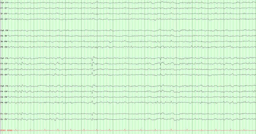
A vertex wave is a central, midline generator, so it appears on both sides at once. The two parasagittal chains carry it simultaneously and symmetrically, and the temporal chains hardly see it. That bilateral symmetry is the finding, not the sharpness.
This is a useful habit in reading sharp transients: before asking how sharp is it, define its field and relationship to state. A true interictal epileptiform discharge may be focal or generalized, so symmetry alone does not make a waveform benign. Here the expected midline maximum, bilateral parasagittal expression, sleep state, and morphology together support a vertex wave.
One vertex wave may be larger on one side. Assess asymmetry across repeated examples rather than classifying a single uneven transient.
N3 is scored from the background voltage, not from a single graphoelement. High-amplitude delta should occupy a substantial share of the epoch.
Spot check Another real sleep page, same longitudinal bipolar layout. Which stage is this?

N3 classification uses the whole epoch: qualifying slow-wave activity must occupy at least 20% of a 30-second adult epoch. This excerpt illustrates the high-voltage, frontally prominent delta to look for; confirm the duration on the full recording.
Spindles may still appear in N3 and are not scored separately. What you should not do is call this N2 because you can still find a spindle, or call it abnormal awake delta. State first, then the voltage makes sense.
Recognizing normal variants
Normal variants can be mistaken for interictal epileptiform discharges. Compare their morphology, field, state, and effect on the background. The drawn pages share one time base and sensitivity, with the channels carrying the finding highlighted; the montage buttons re-derive the same field. The mu rhythm example is a recording.
Mu rhythm
Mu is an arch-shaped central rhythm in the alpha range. It attenuates with movement or the intention to move, often involving the opposite hand, rather than showing the usual eye-opening response of the PDR.
Recognition clues: It lives over the central electrodes, not the occiput, and eye opening does not abolish it. Movement of the opposite hand is the test that separates mu from the PDR.
Wicket waves
Wicket waves are arch-shaped temporal waveforms, often in 6–11 Hz runs during drowsiness or light sleep. An isolated wicket can resemble a spike. Compare it with nearby runs and look for preserved background and no prominent after-going slow wave.
Recognition clues: They come in runs with no after-going slow wave, and the background runs on underneath. The lone wave at 3.9 s on the tracing looks like a temporal spike; the expanded strip below the page shows it has the same shape and size as every wave in the run beside it.
BETS (SSS)
Small sharp spikes (SSS), also called BETS, are brief, low-amplitude transients seen mainly during drowsiness and light sleep. They may be unilateral or independently bilateral, with a broad temporal field and no significant background disruption.
Recognition clues: brief duration, low amplitude, light-sleep context, and preserved background. A small slow component can occur; avoid an absolute “no slow wave” rule.
Rhythmic mid-temporal theta of drowsiness
Rhythmic Mid-Temporal theta of Drowsiness. Runs of monomorphic, flat-topped temporal theta waves (5–7 Hz) lasting several seconds during drowsiness. Typical RMTD remains monomorphic, does not spread, sits in its characteristic drowsy temporal field, and has no clinical correlate.
Recognition clues: The characteristic notched temporal morphology, drowsy state, fixed rate and field, and preserved background support RMTD. Evolution would argue against it, but not every electrographic seizure must evolve.
POSTS and lambda: same shape, different state
Positive occipital sharp transients of sleep (POSTS) occur in light sleep, often in runs. Lambda waves are similar surface-positive occipital transients during awake visual scanning. Use state and behavior to distinguish them.
Recognition clues: Surface positive. POSTS arrive in sleep, usually in trains. Lambda is isolated and tied to visual scanning. Use the Lambda button on the tracing to switch the page. When a patient is awake and looking around, call it lambda; when asleep, call it POSTS.
More variants, side by side
Variant practice: use state and morphology
Use the patient’s state, waveform polarity, distribution, and surrounding background to classify this example. Review the normal variants lesson if you need a reminder.
The technologist documents N1–N2 sleep with eyes closed and no visual scanning. Inspect the posterior transients before choosing a label.
Spot check The technologist documents stable N1–N2 sleep with the eyes closed and no visual scanning. Sharply contoured transients appear over the posterior head. What are they?
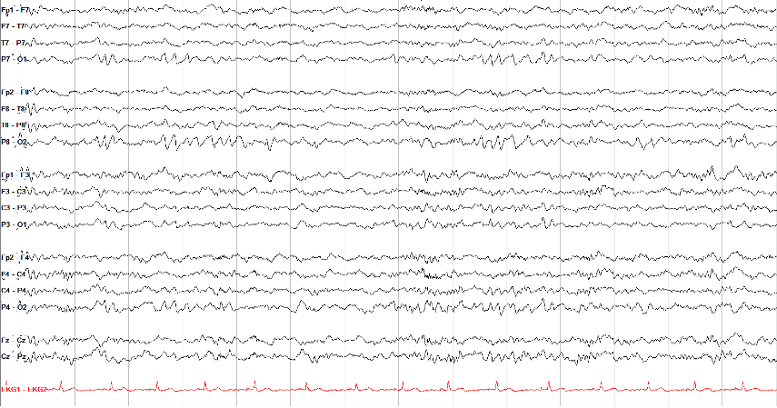
POSTS are normal occipital sleep transients: sharply contoured, surface-positive, often bilateral, and frequently seen in short runs.
Use the expected positive occipital morphology, sleep state, and surrounding background to recognize POSTS. Epileptiform discharges can also occur in sleep and in runs, so those features alone are insufficient.
Lambda waves have a similar occipital positive contour during awake visual scanning. Confirm the behavioral state and timing rather than naming the waveform from shape alone.
Interictal epileptiform discharges
An interictal epileptiform discharge (IED) is a transient with a plausible cerebral field, not simply a pointy waveform. Measure duration first: an EEG spike is 20–70 ms, while a sharp wave is 70–200 ms. Then ask whether the event has a reproducible field, an appropriate phase relationship across channels, a common after-going slow wave, and disruption of the surrounding background. No single feature is mandatory or diagnostic by itself.
Review the same event in three views: identify its morphology, inspect the average-reference field, then compare a second bipolar montage. Follow the actual channel labels in each view.
Select a view to begin.
- Duration: Measure at the baseline crossings instead of judging sharpness by eye.
- Field: Confirm a plausible voltage gradient across neighboring electrodes on more than one montage.
- Context: Decide whether the transient belongs to sleep architecture, artifact, a benign variant, or an abnormal background.
- Repeatability: Find the same morphology and field again before diagnosing from an ambiguous transient.
Where the spike and the slow wave come from
Intracellular recordings from experimental epileptic foci explain the shape of an interictal discharge. During the spike, many neurons in the focus undergo a paroxysmal depolarization shift together: a large depolarization carrying a burst of action potentials, driven by glutamate receptors and voltage-gated Ca²⁺ channels. The after-going slow wave coincides with the hyperpolarization that follows, carried by GABA-mediated inhibition and Ca²⁺-activated K⁺ currents. When that hyperpolarization fails, discharges can merge into a seizure; see Two pathways to an electrographic seizure.
Continue with Interictal epileptiform discharges and Semiology: localizing and lateralizing in Board Review.
Activation procedures
Hyperventilation, intermittent photic stimulation, and sleep may reveal findings absent from the resting record. Describe both the procedure and the EEG response.
Use the laboratory protocol and patient-specific precautions for each procedure.
Hyperventilation (HV)
Typically 3 minutes of deep, rapid breathing (some laboratories extend to 5 minutes when absence seizures are suspected). Hypocapnia produces cerebral vasoconstriction and a fall in cerebral blood flow.
- Normal Response: Generalized slowing (“buildup”), often prominent in children and young adults. Interpret its degree and recovery in context.
- Abnormal Response: Induction of asymmetric focal slowing or generalized 3 Hz Spike-and-Wave discharges (classic absence seizure trigger).
Photic stimulation
Intermittent flashes at rates selected by the laboratory protocol.
- Photic Driving (Normal): Occipital channels synchronize and match the flashing frequency.
- Photoparoxysmal Response (Abnormal): Generalized spike-and-wave or polyspike-and-wave discharges provoked by the strobe. A PPR may be confined to the flash train or persist after it; persistence increases concern but is not required for the definition. A PPR indicates photosensitivity, a largely heritable trait; it is strongly associated with the generalized epilepsies but also occurs in people who never have seizures, so it is interpreted with the clinical history rather than as a diagnosis on its own.
Try both procedures
Read the flash markers along the bottom first. Photic driving is posterior, harmonic to the flash rate, and lacks generalized spike-wave. A photoparoxysmal response adds epileptiform discharges provoked by the stimulus.
Spot check A real photic stimulation page; the flash train is marked along the bottom of the page. What makes a response to the flashes normal rather than epileptogenic?
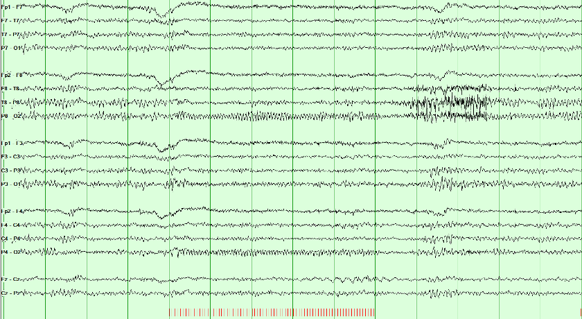
Normal photic driving is a posterior rhythm related to the stimulus frequency or a harmonic. No visible driving response can also be normal. An epileptiform response requires separate assessment.
A photoparoxysmal response is generalized spike-wave or polyspike-wave provoked by flashes. It may remain limited to the stimulus train or continue afterward; persistence strengthens the abnormality but is not required to call a PPR.
Read the stimulus markers first. Timing, distribution, and morphology must be interpreted together: ending with the train does not by itself make an epileptiform response normal.
Combine the activation response with the background and transient assessment. Next, separate continuity from the depth of voltage reduction.
Continuity, attenuation, and suppression
Continuity asks whether activity persists across time. Attenuation and suppression ask how far voltage falls. Keep these four terms in view while you work the cases: they are the vocabulary the later ACNS names depend on.
| Term | What it means |
|---|---|
| Focal attenuation | Regional voltage drop; activity continues on that side |
| Discontinuity | Attenuation or suppression occupies 10–49% of the record |
| Suppression | Voltage below 10 µV. A suppressed background occupies more than 99% of the record. |
| Burst suppression | Suppression below 10 µV occupies 50–99% of the record, alternating with bursts |
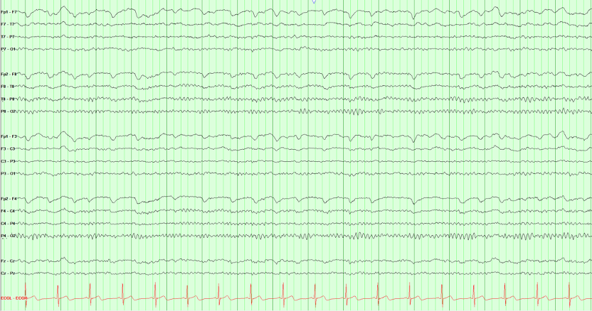
Select a view to begin.
Continue with Coma, cardiac arrest and prognosis and Neonatal seizures in Board Review.
Once voltage over time has a name, ACNS terminology can name the sustained pattern without deciding whether it is a seizure.
ACNS terminology and the ictal–interictal continuum
ACNS critical-care terminology separates description from clinical interpretation. Build the main term from distribution plus pattern, then add modifiers. The name communicates what is on the tracing without presuming cause, seizure status, prognosis, or treatment.
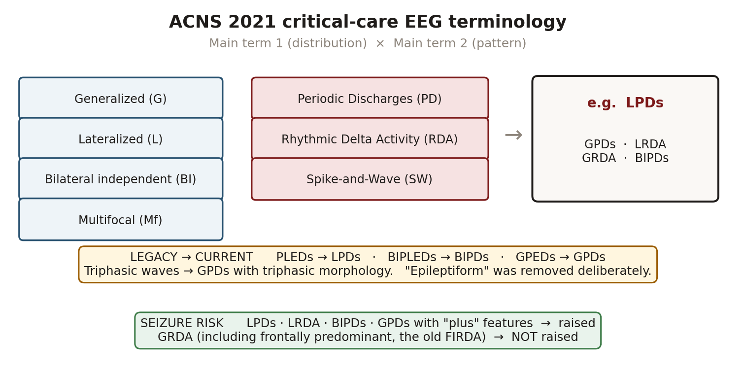
Start with where the pattern is, then whether it is periodic or rhythmic, then add frequency, prevalence, plus-modifiers, fluctuation/evolution, and stimulus relationship.
| Family | Core names | First distinction |
|---|---|---|
| Periodic discharges (PDs) | LPDs, BIPDs, GPDs | Discrete discharges separated by a measurable interval |
| Rhythmic delta activity (RDA) | LRDA, GRDA | Continuous repeating delta without an interval between waves |
- Plus modifiers: +F adds fast activity, +R adds superimposed rhythmic activity to PDs, and +S adds sharp waves/spikes to RDA. Do not use LRDA+R: +R applies only to PDs. For RDA, consider +F, +S, or +FS only when the corresponding feature is present.
- BIRDs: Brief potentially ictal rhythmic discharges are focal or generalized rhythmic activity above 4 Hz, lasting at least 0.5 but under 10 seconds, without a definite clinical correlate. They must not be a known normal/benign pattern or part of burst suppression/attenuation, and must show evolution, resemble this patient’s IEDs or seizures, or have a sharp contour. They are short by definition but carry a strong seizure association.
- SIRPIDs: Stimulus-induced rhythmic, periodic, or ictal-appearing discharges are an umbrella description tied to stimulation, not one morphology or an automatic seizure diagnosis.
- IIC: The ictal–interictal continuum is a risk-bearing gray zone, not a diagnosis by appearance alone. Frequency, plus features, evolution, clinical state, medications, imaging, response testing, and temporal context all matter.
Do not add “epileptiform” back into the legacy names. PLEDs, BIPLEDs, and GPEDs are now LPDs, BIPDs, and GPDs precisely because the descriptive label should not decide ictal significance in advance.
Where a pattern sits
Slowing and periodic patterns
Compare one full-size tracing at a time. The drawn pages share one ten-second time base and sensitivity, and highlight the involved channels, so distribution can be compared without a scale change. The montage buttons re-derive the same field; the LPD example is a recording.
Focal polymorphic slowing
Persistent regional polymorphic delta suggests focal cerebral dysfunction. Structural injury is one possible cause; interpret the finding with clinical history, state, medications, and imaging.
Recognition clues: irregular delta waveforms that persist over a region. The pattern suggests focal dysfunction but does not identify a specific lesion or cause.
Generalized periodic discharges (GPDs)
The synchronized complexes are intentionally higher in amplitude here so their three successive phases are easy to inspect. Triphasic describes morphology, not cause. It can occur in toxic-metabolic encephalopathy and other settings; it is not specific to hepatic encephalopathy.
Recognition clues: A measurable interval separates near-identical complexes, and every chain participates at the same time. GPDs are not automatically seizures; frequency, evolution, plus features, duration, and clinical context determine ictal significance.
Lateralized periodic discharges (LPDs)
Discrete complexes recur over the right posterior temporal and parasagittal chains, with a clear interval between them and no mirror field on the left. LPDs commonly accompany acute focal brain injury and carry a meaningful seizure association.
Recognition clues: Distribution first gives lateralized, and the measurable gap gives periodic discharges. LPDs alone do not prove an electrographic seizure; assess frequency, plus modifiers, evolution, clinical findings, and response over time.
Continue with Periodic patterns by cause and The ictal–interictal continuum and seizure risk in Board Review.
Practice: name the ACNS pattern
Name patterns in ACNS order: distribution first (generalized vs lateralized), then periodic vs rhythmic (measurable gap between complexes vs a continuous run). Compare homologous left and right chains to assess lateralization.
If complexes return to baseline between events and the interval is measurable, the pattern is periodic. A continuous waveform with no gap is rhythmic.
Spot check Repetitive complexes in every chain on a real page. ACNS asks one question before any other. Periodic or rhythmic?
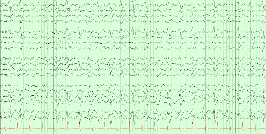
These complexes are periodic because a measurable interval separates successive discharges. Rhythmic waves continue without an interwave interval; they may still cross the baseline.
Generalized distribution plus periodic discharges gives GPDs. The label describes the tracing; it does not determine the cause. A corresponding lateralized pattern is termed LPDs.
Sharpness is not what makes them worrying. Frequency, prevalence, plus-modifiers, fluctuation or evolution, and clinical context determine where a pattern sits on the ictal–interictal continuum. GPDs are not automatically seizures. An electrographic seizure is present if epileptiform discharges average more than 2.5 Hz for at least 10 seconds, or if a pattern shows definite evolution for at least 10 seconds.
LRDA is rhythmic (no measurable gap) and lateralized (larger on one side). Compare each temporal and parasagittal chain with its mirror before picking the maximum.
Spot check Rhythmic delta on a real page, and it is not everywhere. Tap or click the chain where it is largest.
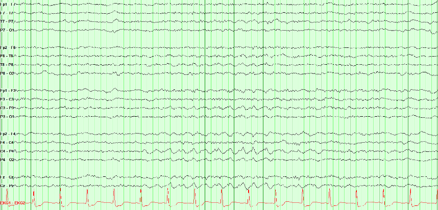
Right lateralized rhythmic delta activity (LRDA). Two things make the call: the waveform is rhythmic (successive waves repeat without a measurable interval between them), and it is lateralized (largest over the right parasagittal region compared with the mirror chain on the left).
Lateralization is always a comparison, never a single-chain judgment. Read each temporal and parasagittal chain against its opposite number, then identify the maximum within the involved hemisphere.
LRDA matters because it carries meaningful seizure association, but plain LRDA is not automatically on the ictal–interictal continuum. Under ACNS criteria, lateralized RDA qualifies for IIC when it is above 1 Hz for at least 10 seconds and has a plus modifier or fluctuation. Distinguish it from polymorphic focal slowing, which is irregular rather than rhythmic and usually points toward focal cerebral dysfunction.
About 1 Hz complexes over one hemisphere with a clear interval between them are lateralized periodic discharges (LPDs). GPDs occupy every chain; chewing is myogenic and time-locked to the jaw.
Spot check Discrete complexes recur about once a second, and they are not everywhere. How should this page be named?

Right posterior LPDs. ACNS naming is distribution, then pattern: the complexes are lateralized (right posterior temporal and parasagittal, no left mirror) and periodic (a clear, near-constant interval). That is LPDs, not GPDs and not a seizure by itself.
LPDs commonly accompany acute focal injury and raise seizure risk. Frequency, plus modifiers, evolution, and the clinical examination decide where they sit on the ictal–interictal continuum. Do not put “epileptiform” back into the name.
Two pathways to an electrographic seizure
ACNS recognizes two routes to an electrographic seizure: (1) epileptiform discharges averaging more than 2.5 Hz for at least 10 seconds, or (2) any EEG pattern with definite evolution lasting at least 10 seconds. Definite evolution is sequential change in frequency, morphology, or location under the ACNS criteria; the pattern does not have to change in all three dimensions. Drag through this left temporal example to see several dimensions change as neighboring cortex is recruited.
Try the evolution pathway: select Onset, then Evolution, then Postictal. Compare frequency, field, and time since onset. Use the slider to inspect the transition between stages.
Read at the green cursor. Stage, frequency, and elapsed time describe that instant. Amplitude is measured across the visible 10-second window, which may include an earlier or later stage. After the seizure ends, postictal time does not extend its duration.
Seizure practice: onset and distribution
Follow seizure activity through time and compare its distribution across channels. Identify the earliest visible change, the sustained field, and any evolution or spread.
After background ends and the seizure begins, follow the full horizontal chain that carries the sustained maximum. Spread into neighboring chains does not erase the original lateral focus.
Spot check This page begins with background, then a right-sided seizure evolves. Tap or click the full horizontal chain that carries the sustained ictal maximum once it begins.
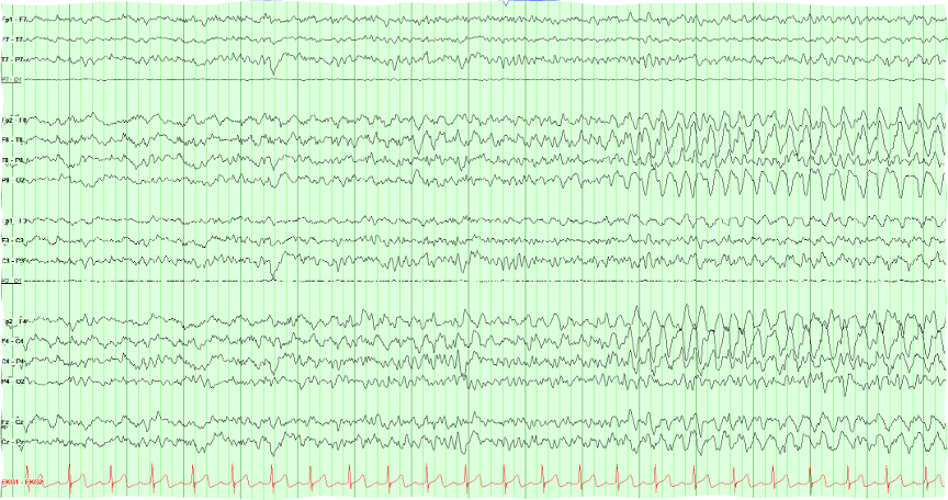
The right lateral chain becomes the sustained ictal maximum. Read its four derivations from top to bottom, then follow them horizontally. The early background is not ictal. After onset, frequency, amplitude, and morphology change as the seizure evolves across the right lateral derivations.
The highlighted chain carries the sustained right lateral maximum. Follow those channels through the event, then compare adjacent chains for spread.
The right parasagittal and midline channels are recruited later. Spread does not erase the earlier and sustained right lateral maximum.
Look for the first generalized complex and compare it with the preceding background. Judge onset, distribution, and evolution together.
Spot check This page starts normal and then does not. Click where the generalized burst begins.
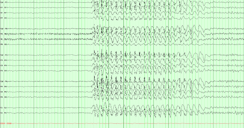
This example shows a generalized spike-and-wave burst with abrupt onset and an organized background before and after. Describe those features before considering syndrome classification.
An organized background between generalized bursts can support a generalized epilepsy syndrome in the appropriate clinical setting. Background appearance alone does not establish the syndrome or exclude a focal onset.
Duration matters, but duration alone does not label the event. A brief generalized spike-wave burst may be electroclinical or subclinical depending on careful testing and video correlation. Absence status epilepticus requires a prolonged generalized epileptiform pattern together with a compatible sustained change in responsiveness or mental state; do not infer it from “a longer-looking burst” without the electroclinical context.
Continue with Seizures on the EEG and Generalized patterns and what they predict in Board Review.
Before accepting an apparent seizure pattern as cerebral, exclude physiologic and technical artifacts that can mimic rhythmicity or evolution.
How ocular artifacts reach the EEG
Artifacts arise from the eyes, muscles, heart, movement, electrodes, or environment. Begin with their distribution and timing, then compare them with video, technologist notes, and auxiliary channels. The eye model below illustrates how ocular fields appear in bipolar channels.
Move the eye and watch the frontal channels
Schematic orientation, not an observer's front view
Choose a blink or move the gaze. The traces show changes from centered gaze; the resting corneoretinal dipole is still present.
How to read this model
The traces show changes from centered gaze. A blink is a brief pulse; the gaze examples show looking away, holding, and returning. Voltages and spatial falloff are illustrative. The blink example includes an upward roll; its degree varies between blinks. The eyelid and rotating globe contribute differently to ocular artifacts. Read the physiology study.
Recognizing common artifacts
Eye blinks
The eyeball behaves as a dipole: the cornea is relatively positive and the retina relatively negative. Eyelid movement over the cornea contributes to the blink potential, which is commonly positive and maximal at Fp1/Fp2. Upward eye rotation may accompany eye closure, but does not explain every blink. In an Fp1–F3 derivation, Fp1 is Input 1; a relatively positive Input 1 produces a downward deflection when negative is displayed upward.
Recognition clues: Look for a bilateral frontal transient time-locked to blinking, usually smaller in more posterior channels. Confirm with eye channels or video; frontal distribution alone does not prove artifact.
Lateral eye movements
Left gaze makes the field near F7 relatively positive and near F8 relatively negative; right gaze reverses the pattern. Display direction depends on each channel’s subtraction. Brief muscle spikes may accompany saccades.
Recognition clues: The mirror-image frontal field matches the corneoretinal dipole and is time-locked to eye movement on video or eye leads. Watch for lateral rectus spikes at each onset.
Muscle (EMG) artifact
Extremely high-frequency, narrow, jagged buzz caused by jaw clenching, chewing, or tension. Classically maximal in temporal channels (T7/T8). Oversmoothing with filters to remove this can artificially round the muscle spikes, causing them to look like cerebral Beta waves.
Recognition clues: Individual motor-unit spikes are visible in the expanded inset. Filtering them rounds them off until they look like cerebral beta, which is the trap.
60 Hz line interference
A regular fast artifact from mains interference, poor or unbalanced electrode contact, nearby equipment, or grounding problems. First inspect electrodes and the environment. A notch filter may reduce residual interference but can distort activity near the filtered frequency and should not replace troubleshooting.
Recognition clues: regular mains-frequency activity. A contact problem may affect channels sharing one electrode; interference can also be widespread. Check the contacts, leads, and environment.
Artifact practice: field and timing
Read distribution before shape, as in the artifact gallery. Frontal drop-off points to the eyes. Temporal myogenic bursts follow jaw movement. Mechanical rhythms lock to devices on video and non-cerebral channels.
Brief, bilateral, frontal deflections with an untouched posterior background point to the corneoretinal dipole, not a cerebral discharge.
Spot check Brief, repeated, frontally maximal deflections on a real page, and the posterior background is untouched. What are they?
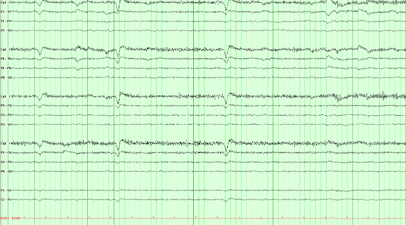
The positive cornea and negative retina form a dipole. Eyelid movement and accompanying eye rotation can produce a brief, bilateral frontal potential, usually largest at Fp1/Fp2.
Three features identify it and all three matter: the distribution is frontal and drops away immediately, the events align with blinking on video or eye leads, and the background elsewhere is unaffected. The repeated shape is compatible with blinks, but epileptiform discharges can also be stereotyped, so stereotypy is not the discriminator.
Eyelid flutter can mimic frontal rhythmic delta. Check its timing against video or eye channels and compare the field across the scalp before assigning a cerebral pattern.
Rhythmic alone is not ictal. Check video, technologist notes, and non-cerebral channels for a mechanical source before calling a seizure.
Spot check A rhythmic pattern is running through this record. Before calling it a seizure, what should you check?
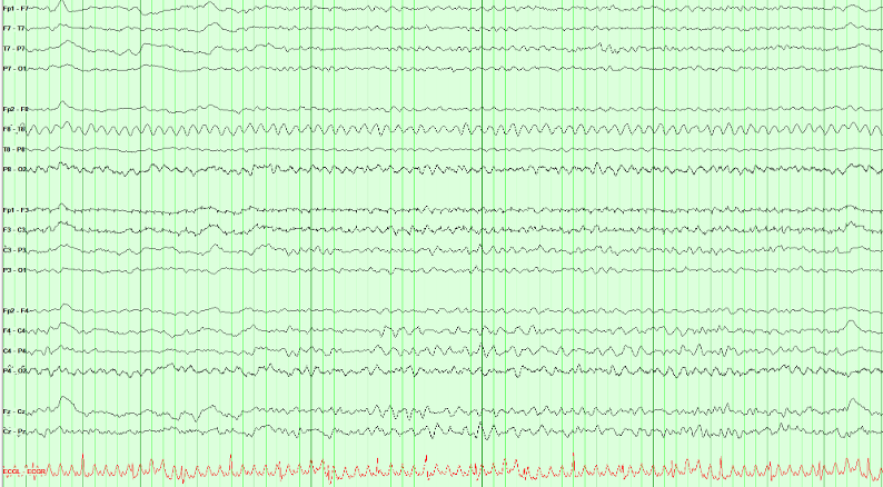
Mechanical devices can drive a highly regular rhythm through the patient and electrode array. A percussor, ventilator, or vibrating bed may produce a fixed rate with no physiologic field, no independent cerebral evolution, and exact temporal coupling to the device.
Lack of evolution alone does not exclude an electrographic seizure, because qualifying epileptiform discharges above 2.5 Hz for at least 10 seconds provide the other pathway. Here, however, the waveform is not an epileptiform discharge and the bedside/video correlation identifies its mechanical source.
Compare the pattern with ECG, respiratory, or movement channels when available. Review video and technologist notes for time-locked equipment or patient movement.
A ~1 Hz cadence with EMG needles densest in the temporal chains, a quiet EKG, and no cerebral field is chewing artifact, not periodic discharges or a seizure.
Spot check High-amplitude bursts march through this page about once a second. The EKG underneath is regular. What is contaminating the record?

Chewing is muscle, at the frequency of the jaw. Each burst is packed with high-frequency motor-unit spikes, maximal in the temporal chains, and the EKG is unaffected. Ask the technologist to pause chewing, or watch the video: the page quiets when the jaw does.
The burst rate follows chewing. Temporal muscle distribution, high-frequency components, and a matching jaw movement support artifact; regular repetition alone does not establish a cerebral periodic pattern.
Artifact Hunter: correct the source
Artifact Hunter: Clean the Trace
Click a channel to see what contaminates it, then use the controls to address the source. Click a control again to restore the artifact for comparison. Recognizing ECG leaves the recorded signals intact.
From tracing to report
A report should connect the EEG description to the clinical question. Include relevant state, medications, stimulation, behavior, and technical limitations. Use the sequence below as a writing guide.
Clinical report template
- Study details
- Start time, recording type, duration, electrodes, montages, and any technical limitations.
- Clinical history
- @AGE@ with possible seizures. Age and the clinical question. Note recent seizures, temperature, and other major confounders when known.
- CNS-active medications
- Sedation, antiseizure medications, and other CNS-active drugs that change the tracing.
- Recording day
- Day header for serial or long-term recordings. Repeat the fields below for each day.
- Background
- Describe organization, symmetry, predominant frequencies, anterior–posterior gradient, PDR frequency and reactivity, variability, and stimulus reactivity.
- Sleep
- Architecture and state changes, separate from the waking background. State whether sleep was captured.
- Continuity and voltage
- Whether activity persists across time, and how far voltage falls (attenuation or suppression).
- Slowing
- Distribution and prevalence. Do not bury this inside the background sentence.
- Activation procedures
- Hyperventilation and photic stimulation: performed or not, and the response.
- Epileptiform, rhythmic, and periodic patterns
- IED morphology, field, location, and abundance. Name rhythmic or periodic patterns with ACNS terms and modifiers.
- Seizures and clinical events
- Onset, duration, evolution, and spread. Review video and technologist notes. State whether an electrographic correlate was present and whether awareness was tested.
- Quantitative EEG
- Record quantitative EEG findings if they were reviewed. If QEEG was not part of this study, say so.
- ECG
- Heart rate and rhythm from the EKG channel. Confirm ECG artifact on the scalp against this channel.
- Impression
- Prioritize the main findings, explain their clinical significance, compare with prior recordings when available, and state meaningful limitations.
Local Epic reporting templates and daily checklists live on the Epilepsy Rotation resources page.
Review before signing: the impression should summarize the findings and their significance without introducing observations absent from the description.
Continue with Recording technique for the full reporting framework.
Practice before you finish
Write a short report from a case
Use only the facts below. This is a fictional teaching case; do not enter patient information.
Case facts
- Technically adequate, 30-minute routine scalp EEG for episodes of staring.
- Awake background is organized and symmetric. A 9 Hz posterior dominant rhythm attenuates with eye opening.
- N2 sleep is recorded with symmetric spindles and K-complexes.
- No focal slowing or interictal epileptiform discharges are seen. No clinical event or electrographic seizure occurs during the recording.
- Photic stimulation produces no abnormal response. Hyperventilation was not performed; the reason is not supplied. Medication history and prior EEGs are unavailable.
Model answer and self-check
Background and sleep
The awake background is organized and symmetric, with a 9 Hz posterior dominant rhythm that attenuates with eye opening. N2 sleep is present with symmetric spindles and K-complexes. No focal slowing or interictal epileptiform discharges are seen. Photic stimulation produces no abnormal response; hyperventilation was not performed. No clinical event or electrographic seizure was captured.
Impression
Normal awake and asleep EEG in this teaching case. No epileptiform discharges or seizures were recorded during this 30-minute study. A normal interictal EEG does not exclude epilepsy or determine whether the reported staring episodes were epileptic.
Check your draft: Did it state the recording state, PDR and reactivity, N2 features, activation procedures, and the findings that were absent? Does the impression summarize only what the description supports, without inventing medication details or prior EEG results? It is fine if your wording differs from the model.
Clinical limit: a normal interictal EEG does not exclude epilepsy. ACNS Guideline 7.
After the last lesson
Take the post-test
Finish the course with the post-test. It uses the same study code as your pre-test so the two sets of answers can be paired. If you skipped the pre-test, the post-test is still useful.
The test link is loading.
Submit the Google Form, then come back here. Opening the link alone does not record a response.
Use a code saved on another device
Place the 10–20 electrodes
Put each electrode where it belongs until you can find every site without the guides. The nasion, inion and ear points are drawn on the head, and the 10–20 spacing lines can be switched on whenever you need them.
Choose an electrode, then click its position on the head. With the keyboard, focus the head, move the crosshair with the arrow keys (Shift for small steps) and press Enter to place.
This view is a schematic on an idealized head; it supplements supervised technologist training and local protocol. Next, the electrodes are connected into channels.